


Earlier this week Patrik Berglund, Xeneta CEO and Co-founder presented our quarterly ocean freight rates in a LIVE webinar. He did an analysis of the main trade routes Asia - Europe (in/out) as well as the trans-Pacific where he shed light on how container rates in Q2 2017 have fluctuated. In addition, he did a 12-month analysis of historical rates for the spot and long-term market and drew correlations between the two markets to give indications of what can be expected in Q3.
Webinar - Ocean Freight Rates Review
- Presentation transcript: Read below (or download full transcript in PDF format)
- Live Q&A session: Read answers to common questions from the webinar
Presentation Transcript
[Patrik Berglund]:
Today's Agenda
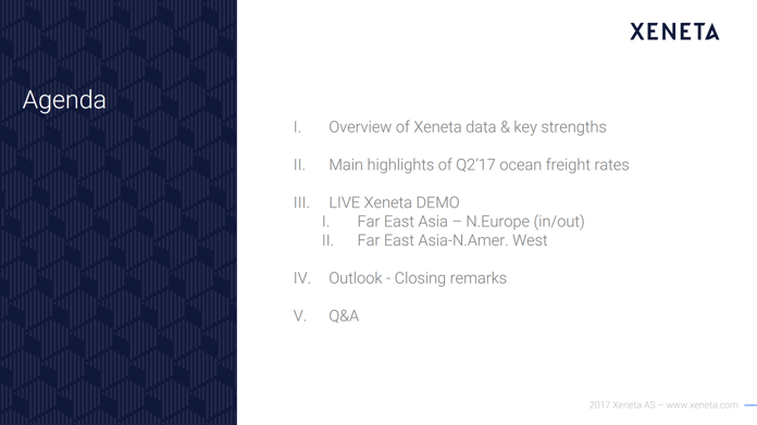
[02:33] I just wanted to mention that we had our customer webinar earlier today, where we go more in‑depth into findings in our data and more in‑depth analysis.
[02:51] We're going to use the actual application today and go through these different corridors and we will take questions. If there's certain aspects missing, I just wanted to make sure that it's a possibility for our customers to go more in‑depth on a more dynamic session as well. With that in mind, let's start with the first point.
[03:13] Xeneta is an Oslo‑headquartered company, and we've got offices in Boston and Hamburg. We collect freight rates and build that up into a database that allows shippers, BCOs, NVOCCs to benchmark and extract market intelligence from our online application. We've got more than 700 companies worldwide connected to this tool and more than 2,000 users.
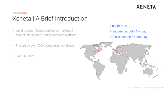
[03:35] Now, the key thing and whole crux of Xeneta is this database of actual contracted rates. Today, we have a database of more than 35 million rates on 160,000 different port pairs. But we're importing every month now between 2 and 3 million rates into our tools, so this database is still rapidly growing.
[04:02] This means that you have fresh, relevant, accurate real data available when logging in. Xeneta is a neutral company, which is key in order to service all these different stakeholders. There is no ownership stake in our company from the buying side or the selling side of the industry.
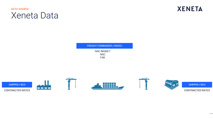
[04:24] The crucial thing to understand is where do we source this data from. We source it either from the shipper, or the consignee, the one that owns the contracts. We also source data coming from NVOCCs, but we bracket it into Named Account Basket, Named Account, and Freight All Kind rates. Whatever we have of data, users are able to filter out and segment the data they would like to review.
[04:50] With this in mind, I want to go directly to the tool, and I'm going to use the tool in itself. When I log in, it looks like this. I can immediately start my search for the first corridor that we're going to have a look at today. It's going to be the corridor that belongs to Shanghai to Hamburg.
[05:09] I'm going to immediately roll up in this Geo‑Hierarchy, so that we pull data from China Main ports rather than just Shanghai, and I select that. I do the same on the European side with Hamburg, letting it load the data, and then switching to North Europe Main on the destination side.
[05:33] This will show me a 12‑month historical overview of 20‑foot rates between China Main ports to North Europe Main ports. I can easily switch to 40‑foot containers by clinking it on the bottom here, and then see how the markets move for 12 months.
[05:51] You have a chart with US dollars on the Y‑axis and a 12‑month historical overview on the X‑axis. You see on the selection here that we're currently looking at the market average for a 40‑foot container. It's a blended value of contracts, so what I immediately would need to do is to select the contract duration that I want to have a look at.
[06:17] Since this webinar is mainly centered around Q2, I could have chosen a timeline to only review Q2, but I think for the listeners and the viewers out there it makes much more sense to see the quarter in a longer time perspective.
[06:35] For this webinar, I've deliberately chosen a 12‑month period. You will see in this chart that this corridor is highly volatile, but for the duration of Q2 it's been some Geo rise that has declined, but quite stable compared to the last 12 months.
[07:01] I want to do one more thing for the short‑term market on this one. I want to go back all the way to beginning of January to give you some perspective on what is a high or a low market on this corridor for a 40‑footer.
[07:13] I just changed the calendar here to pull data from first of January 2016, all the way up until today. Here you will start to see some interesting movements. You will see that we went into 2016 on this Chinese New Year spike that just quickly diminished, all the way until March, where the average sat at $403.
[07:41] Then a few months later, you had the peak, here in July, on 1,945. This shows us that the market now, over Q2, this stabilized period here, it's actually quite on par with what we've seen for the last nine months or so.
[08:04] The short‑term market is incredibly important to understand in relation to the long‑term market. You will, here, clearly see a market that has moved down, and then picked up. You would expect then to see the same pattern in long‑term contracts, but with a slight delay.
[08:27] If I select now long‑term contracts by clicking far left here, you will see that the platform pulls up all long‑term contracts between China Main to North Europe Main, and shows you the pattern. It shows that it's going down, and then later in time it starts to increase simple because the contracts on the long‑term market expires less frequently.
[08:54] In our tool you can, of course, also select the market low so that can see the spread of the market. You see some of the same pattern there. Going out of Q2, the long‑term market sat at $1,380 on the average and $700 on the lower end.
[09:19] Let me see. If we do one more thing here, another important element to understand is that we can further slice the data so that you can see what has happened within the last three months. If I click the button to the far left, what the platform will do is that it will eliminate all the old long‑term contracts every single day.
[09:45] Then you see that the market moves more aggressively upwards earlier in time than what we just looked at when we had all contracts selected. Every single date it looks a maximum of three months back, pulls all the long‑term contracts that are newer than three months, and shows forward in time.
[10:08] This shows that the long‑term market for China Main to North Europe Main has moved substantially up over the last 9 months, 12 months. You will see that it bottomed out in June last year at $616, and then going out of this quarter it was on $1,470 on average. You also see that it continued to pick up in July.
[10:33] One last thing I want to also show in this one is the ability to look into the future in terms of what has already been contracted. Now with the selection of a rolling three‑month average, it will still look three months back for any given date in the future, and only pick up the old contracts.
[10:53] This indicates to us that the market is continuing to pick up, and that long‑term contracts are expected to continue in increase. The same development that we saw during Q2 and for the last 12 months is expected now, based on what is signed and agreed today, to continue.
[11:16] I'm then going to cover the reverse corridor. I'm going to simply click this button here, which reads reverse lane. We're going to look at North Europe Main to China Main ports. This is one of the interesting corridors, to be honest, for the last eight, nine months. It's historically one of the corridors that has been fairly stable on the short‑term market, as well.
[11:41] If I go back to beginning of January 2016, you will see that it's been fairly flat for a longer period of time, down here. Then you have these well‑known increases that we see, especially in Q2, but as you can see from this data we started picking up the increase already back in September, going into October, November, December.
[12:06] Then, as the new alliances came into play, we had this substantial bump in the market. So in April, during Q2, the market average had a peak of $2,009 for a 40‑footer on the short‑term market, which compared to a year ago is almost 4x.
[12:26] Then, as the alliances stabilized, the new networks were introduced and there was less reports of shortage in volume, you will see how quickly the short‑term market has moved down again. What's interesting here is that if we switch to the long‑term market you will see some of the same movements. I've already selected a rolling three‑month average, since it's a more accurate reflection of the market.
[13:02] You will see the uptick here, and as I mentioned, the long‑term market moves with a delay compared to the short‑term market. You will see here the market going up on July as another increase from $712 to $825, but during Q2 the market went from $511, exiting Q1, all the way up until $712. This is continuing to trend upward.
[13:32] What you also can say here is that we expect the market either to go a little bit more up or stabilize before we start seeing the decline that we've seen in the short‑term market. Again, that's why these two data sets are so incredibly important in combination, rather than just having one of them at your disposal.
[14:01] Let me do one more thing to make it vividly clear what we're doing. If I go to the reverse lane again, back to China Main to North Europe Main, I want to do one more point here. We covered this one on the short and the long‑term. I want to show the data behind, to make this point clear.
[14:20] I want to show you this chart, very briefly. This is one port combination within China Main to North Europe Main ports, 40‑footer, and I've chosen all the data going back to 2014. Again, it's a US dollar Y‑axis, and then you have a timeline at the bottom.
[14:39] In this scatter plot you see all the raw data. The length of the line here represents long‑term contracts. You'll see here long‑term contracts reaching out well into Q2 of 2018. You will see, for instance, here, back in 2014, how the short‑term market sat above the long‑term market.
[14:58] You will see that when you came to year‑end for 2014, the long‑term contracts continued into 2015 on this level, while the short‑term market plummeted. This is relevant in terms of these two markets moving in relation to each other.
[15:15] When we saw this situation, we knew that coming year‑end 2015, if the short‑term market hadn't then picked up before 2015, long‑term contracts would move in relation to these short‑term ones. You see that going into 2016. All the long‑term contracts, or the vast majority of them, moves down, and the short‑term market has this Chinese New Year's spike, only for it to plummet back down into March 2016.
[15:48] We started looking at the chart from the 1st of January, 2016. Here you can clearly see the same pattern. Short‑term rates, spot market moving up. As these long‑term contracts comes to an end, both year‑end, and then the prolonged contracts, then you see that they move after.
[16:09] This is important to understand because this is the data behind the chart that we just looked at, either this one or short‑term. This is what it pulls, all the raw data behind, and shows the short‑term market movements and long‑term market movements.
[16:27] With this in mind, I will go to China Main to North America West Coast. Let's pull that one up. Let's start by looking at the short‑term market. Again, I want to do a prolonged period of time. I want to do 1st of January until today. You will see here that it has a very different pattern to what we looked at for Asia‑Europe and Europe‑Asia.
[16:56] This has an increase, and then a substantial decrease. This decrease has gone on since almost the beginning of the year, where the market has moved on short‑term 40‑foots and drove angle boxes from $2,318 on the peak, down to $1,369 end of Q2. Again, a very volatile corridor, but if we switch to the long‑term market we should start to see some patterns here, as well, in terms of movements.
[17:39] Now it's loading all long‑term contracts China Main to North America West Coast. I'm going to do a rolling six‑month average here. There's the rolling three‑month average, as well, which has some substantial increases and decreases. If you look at this one, it shows some of the same patterns. Long‑term contracts going down, then moving up, and then somewhat down again.
[18:03] The GRIs that they've introduced month‑on‑month, and you saw in the short‑term market, hasn't been very successful since we went into 2017. If I look at contracts going into the future, based on what's negotiated for the last six months, you will see that it stays somewhat flat, which is why it declined looking into October. Old contracts expiring, new ones coming into play.
[18:33] If you look at the same one with the last three months' selection, you will see that market continues to drop more significantly, which is more reflecting the short‑term market movements as we're currently seeing.
[18:45] All of this data is instantly available and accessible through our application. The importance that I hope I got demonstrated here today is how to see not only one quarter isolated, and the movements, and the hard‑used dollar values on a daily basis, but how they move in relation to each other.
[19:08] With that, I will end our live demonstration for today. Kathy, I'll leave them over to you.
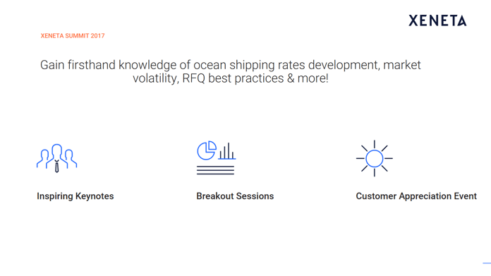
Katherine: [19:23] Thank you, Patrik. Thanks. Before we jump into our question and answer section, I wanted to give a little bit of information about our first annual Xeneta Summit that we're going to host this autumn, in September, in Hamburg. It is a customer‑only event.

[19:42] As I mentioned, it's the first time that we're doing it. Just to give you a bit of information of what you can find there for customers, we will be hosting a two‑day event where we're going to have keynote sessions, breakout sessions, and of course some fun for networking amongst all the users of Xeneta.
[20:02] What's interesting is the information that Patrik just talked about today, we will go really in‑depth then and have some full analysis on that information at the summit. On the next slide, I'll give you a sneak peek of some of the topics that we're going to be covering with our ocean freight experts.
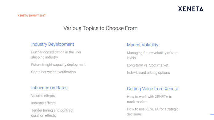
[20:21] Patrik will be there, our other co‑founder Thomas, Michael Braun, who's also an ocean freight expert, as well as some other people within Xeneta. We're going to talk about market volatility, long‑term contracts versus spot market. We're going to dig real deep into our data, find what type of influences there are on rates, for example, volume or industry. They'll give you some tips on when to be negotiating, for example.
[20:49] We'll also be showing the next version of our user interface. We'll also show you how to best use the platform, how to best extract information, how to be able to do some of these analyses that Patrik did. What's also interesting is that we'll have some panel sessions, and we'll have some discussions. The best is also to meet peers that are also using the platform, and learn best practices.
[21:15] That is in September. It is a customer‑only event, so I guess it's a bit of a teaser for those that aren't yet customers. We're quite excited about it. If you're interested, of course, reach out to us.
###
Common Questions From The Webinar Q&A
Q1. Is it preferable to agree on a three‑month contract or month‑by‑month?
A1. We see, actually, a pattern of more and more companies going on shorter contract durations, not necessarily month‑by‑month, but annual contracts are maybe shifted to quarterly or six‑month, or an annual contract with quarterly reviews, using, of course, our data to review that to see if the market went up, or how much did it move down with.
If you allow me to, bear with me, I will actually pull up a slide that we used in our customer session earlier today that I think might be of interest. I'm going to do that, but bear with me. I think it gives a sneak peek of what we're showing there, as well.
I'm going to do this one. This is China Main ports to North Europe Main ports. This is the short‑term market in black and the long‑term market in orange. Obviously, there's simple things to derive here immediately, it's only a short period of time where it was more competitive, or beneficial, to be in the short‑term market over the last 18 months.
That has changed dramatically compared to what we saw in 2015, for instance, where almost the full year was better off being in the short‑term market than in the long‑term contract. By long‑term contracts, to us that's more than a three‑month duration. Really, what I think is the best approach to this is to keep tabs on where the market is trending.
Immediately now, when you see the market here has been trended upwards for a long period of time, then you know that it's the short‑term market that will move first, hence it will be this delay in the long‑term market that makes it beneficial to go long.
Then, if the market turns, then it moves down, think about the Europe to Asia chart that we looked at in our tool. Now the market is moving down on that on the short‑term, so if you have the abilities to switch and sit in the short‑term market on that corridor, that would definitely be the most competitive prices you could reach, as for now.
This keeps on changing. Very often it's vice‑versa, so keeping tabs on this, and having this insight is exactly what we provide you with.
Q2. Can we break out any contract movements on a commodity basis, rather than an aggregate level?
A2. Yes. I don't think Kathy specifically mentioned that, but that is stuff we do for our customers. That's insights we will share in our summit in Hamburg.
Q3. How does chemical companies stack up to automotive companies, and so forth?
A3. As for now, in this session, we're not presenting any insights on that, but in our summit or in customized analysis we do pull out that, because all the data, every single rate point, has a volume attached, it has, also, industry attached to it. We could basically answer any questions in that direction as long as is the data is densely enough on the different trade routes that we have.
Q4. Which factors influence ocean freight rates?
A4. There's a few things that are basic. Obviously, oil prices influence some, but the key, key thing that we see drive prices up and down is capacity versus utilization.
If we go back to the period before March '16, there was structural overcapacity and prices for the two years before that was trending down, down, down. Then they managed to pull out more capacity.
Also, on the European to Asia one, when they restructured their alliances there was a lot of equipment shortage. Slots were very difficult to get on the vessels, then prices spikes immediately. If there's spare capacity, then prices drops. That's the main key driver that we see.
Q5. Does freight‑rate volatility affect container rates? How has the general rate increase on European routes affected container rates?"
A5. The first part of the question, "Does freight‑rate volatility affect container prices?" whether that's the actual procurement of the container, in itself, that's not our domain. I'm struggling to interpret the question any other way, but I can cover the GRI ban on European routes.
The only change we've seen for from some of the carriers on that is that they earlier on announces their GRI, and then they set that as a roof where they can only go down from, and they can't do a mid‑month GRI, even though we see that's still happening. That's one of the tricky things about this industry.
When we read about this new rules being introduced, we found it difficult to see how the laws would be enforced. We're still picking up patterns and movements from our data that doesn't really correlate with how these regulations should be working, but we see some changes from some of the carriers without hanging anyone out there to dry. I'm going to limit it to that.
Q6. Does Xeneta have FMCG as an industry?
A6. Yes, we have. Every company that joins Xeneta, we tag them with one or more industries so that we can segment the data coming from them.
Q7. What are your weakest trade lane freights?
A7. This is easily addressable. Our data correlates very highly to the global trade patterns. If you have Far East Asia to Europe, Europe‑Asia, Far East Asia to US, Far East Asia to the South America, where there are some of the biggest trade routes in the world, those will be densely populated.
If you look from Shanghai to Mombasa, or Turkey to Sydney, we would have less data, simply because it's less companies moving cargo on those routes. That being said, you will find very exotic combinations in our tool, whether it's Tokyo to Brisbane, or whether it's Turkey to Middle East. With 160,000 different combinations, more or less every relevant trade route in the world is covered.
We also disclose the data density in our tool, which means that if you segment out long‑term contracts going between Santos to Helsinki, you will see that there's less data behind it, but it's more than you have just looking at your own contracts.
###
If you missed any our webinars – or simply want to refresh your memory – you can access all of them on demand here.
See you next time!